pacman::p_load(tidyverse, jsonlite,
tidygraph, ggraph)Take-home Exercise 02 - Data prep
1. Getting Started
1.1. Loading R packages
In this take-home exercise, the 4 packages below will be used:
2. Importing knowledge graph data
For the purpose of this exercise, MC1_graph.json file will be used. In the code chunk below, fromJSON() of jsonlite package is used to import MC1_graph.json file into R and save the output object
kg <- fromJSON("C:/Cindy-2312/ISSS608-VAA/Take-home_Exercise/MC1_release/MC1_graph.json")2.1. Inspecting the data structure
Before preparing the data, it is always a good practice to examine the structure of kg object. In the code chunk below str() is used to reveal the structure of kg object.
str(kg, max.level = 1)List of 5
$ directed : logi TRUE
$ multigraph: logi TRUE
$ graph :List of 2
$ nodes :'data.frame': 17412 obs. of 10 variables:
$ links :'data.frame': 37857 obs. of 4 variables:3. Extracting the edges and nodes table
Next, as_tibble() of tibble package package is used to extract the nodes and links tibble data frames from kg object into two separate tibble data frames called nodes_tbl and edges_tbl respectively.
nodes_tbl <- as_tibble(kg$nodes)
edges_tbl <- as_tibble(kg$links)
3.1. Initial EDA
It is time for us to apply appropriate EDA methods to examine the data. In this code chunk below, ggplot2 functions are used the reveal the frequency distribution of Edge Type field of edges_tbl.
ggplot(data = edges_tbl,
       aes(y = `Edge Type`)) +
  geom_bar()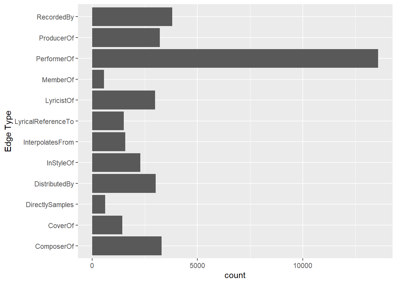
On the other hands, code chunk below uses ggplot2 functions to reveal the frequency distribution of Node Type field of nodes_tbl.
ggplot(data = nodes_tbl,
       aes(y = `Node Type`)) +
  geom_bar()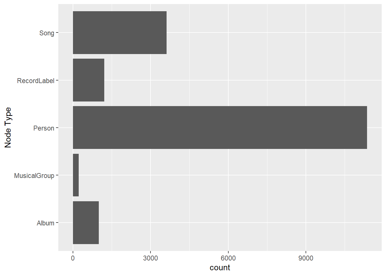
4. Creating knowledge graph
4.1. Mapping from node id to row index
Before we can go ahead to build the tidygraph object, it is important for us to ensure each id from the node list is mapped to the correct row number. This requirement can be achieved by using the code chunk below.
id_map <- tibble(id = nodes_tbl$id,
                 index = seq_len(
                   nrow(nodes_tbl)))
4.2. Map source and target IDs to row indices
Next, we will map the source and the target IDs to row indices by using the code chunk below.
edges_tbl <- edges_tbl %>%
  left_join(id_map, by = c("source" = "id")) %>%
  rename(from = index) %>%
  left_join(id_map, by = c("target" = "id")) %>%
  rename(to = index)
4.3. Filter out any unmatched (invalid) edges
edges_tbl <- edges_tbl %>%
  filter(!is.na(from), !is.na(to))
4.4. Creating tidygraph()
graph <- tbl_graph(nodes = nodes_tbl,
                   edges = edges_tbl,
                   directed = kg$directed)
class(graph)
[1] "tbl_graph" "igraph" 5. Visualizing the knowledge graph
set.seed(1234)5.1. Visualising the whole graph
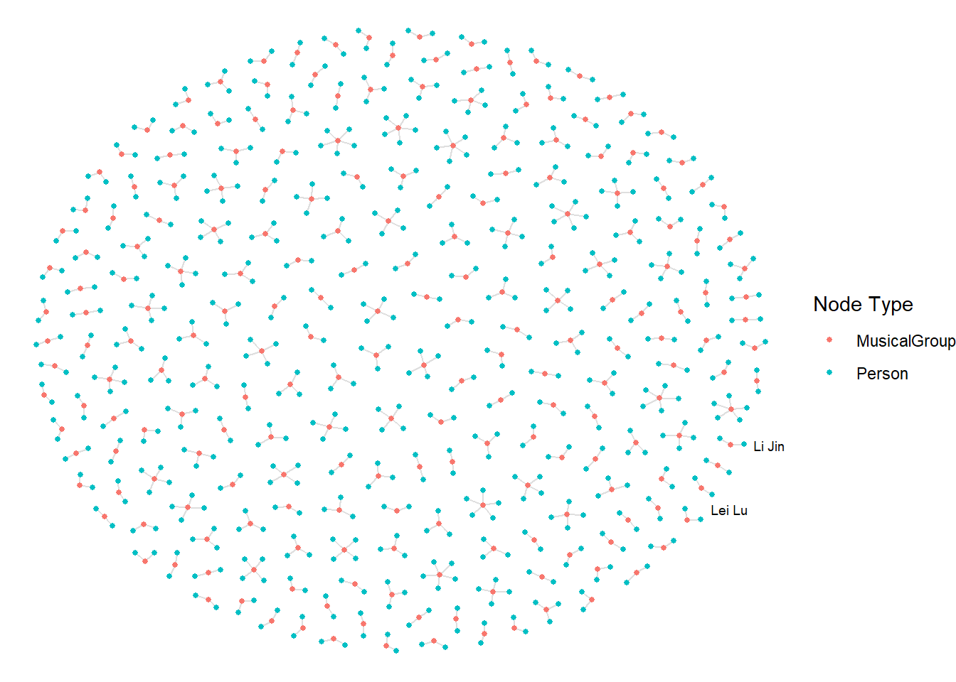
5.2. Visualising the sub-graph
In this section, we are interested to create a sub-graph base on MemberOf value in Edge Type column of the edges data frame.
Filtering edges to only “MemberOf”
graph_memberof <- graph %>%
  activate(edges) %>%
  filter(`Edge Type` == "MemberOf")
Extracting only connected nodes (i.e., used in these edges)
used_node_indices <- graph_memberof %>%
  activate(edges) %>%
  as_tibble() %>%
  select(from, to) %>%
  unlist() %>%
  unique()
Keeping only those nodes
graph_memberof <- graph_memberof %>%
  activate(nodes) %>%
  mutate(row_id = row_number()) %>%
  filter(row_id %in% used_node_indices) %>%
  select(-row_id)  # optional cleanup
Plotting the sub-graph
ggraph(graph_memberof,
       layout = "fr") +
  geom_edge_link(alpha = 0.5,
                 colour = "gray") +
  geom_node_point(aes(color = `Node Type`),
                  size = 1) +
  geom_node_text(aes(label = name),
                 repel = TRUE,
                 size = 2.5) +
  theme_void()
Warning: ggrepel: 789 unlabeled data points (too many overlaps). Consider
increasing max.overlaps