Take-home Exercise 01

Author

Cindy TA

TAKE-HOME EXERCISE 01 - PHASE 1

1. Introduction

1.1. Setting the scene

A local online media company that publishes daily content on digital platforms is planning to release an article on demographic structures and distribution of Singapore in 2024.

1.2. The task

In this take-home exercise, we are assuming the role of the graphical editor of the media company,and are tasked to prepare at most three data visualisation for the article.

2. Getting Started

2.1. Importing packages and libraries

In this project, the below R packages will be used:

ggrepel - Provides geoms for ggplot2 to repel overlapping text labels, making charts more readable
patchwork - Helps combining multiple ggplot2 plots into a single layout
ggthemes - Offers additional themes, scales, and geoms for ggplot2 to enhance visualization styles
hrbthemes - A set of typography-centric themes and utilities for ggplot2 (nice fonts and spacing)
tidyverse - Core collection of R packages designed for data science
ggplot2 - The main R package for creating static graphics using the grammar of graphics framework

pacman::p_load(ggrepel, patchwork, 
               ggthemes, hrbrthemes,
               tidyverse, ggplot2)

2.2. Importing data

The dataset shared by Department of Statistics, Singapore (DOS), Singapore Residents by Planning Area / Subzone, Single Year of Age and Sex, June 2024, is used

pop_data <- read_csv("data/respopagesex2024.csv")

Rows: 60424 Columns: 6
── Column specification ────────────────────────────────────────────────────────
Delimiter: ","
chr (4): PA, SZ, Age, Sex
dbl (2): Pop, Time

ℹ Use `spec()` to retrieve the full column specification for this data.
ℹ Specify the column types or set `show_col_types = FALSE` to quiet this message.

head(pop_data)

# A tibble: 6 × 6
  PA         SZ                     Age   Sex       Pop  Time
  <chr>      <chr>                  <chr> <chr>   <dbl> <dbl>
1 Ang Mo Kio Ang Mo Kio Town Centre 0     Males      10  2024
2 Ang Mo Kio Ang Mo Kio Town Centre 0     Females    10  2024
3 Ang Mo Kio Ang Mo Kio Town Centre 1     Males      10  2024
4 Ang Mo Kio Ang Mo Kio Town Centre 1     Females    10  2024
5 Ang Mo Kio Ang Mo Kio Town Centre 2     Males      10  2024
6 Ang Mo Kio Ang Mo Kio Town Centre 2     Females    10  2024

2.3. Exploring data

summary(pop_data)

      PA                 SZ                Age                Sex           
 Length:60424       Length:60424       Length:60424       Length:60424      
 Class :character   Class :character   Class :character   Class :character  
 Mode  :character   Mode  :character   Mode  :character   Mode  :character  
                                                                            
                                                                            
                                                                            
      Pop              Time     
 Min.   :   0.0   Min.   :2024  
 1st Qu.:   0.0   1st Qu.:2024  
 Median :  20.0   Median :2024  
 Mean   :  69.4   Mean   :2024  
 3rd Qu.:  90.0   3rd Qu.:2024  
 Max.   :1180.0   Max.   :2024

unique(pop_data$PA)

 [1] "Ang Mo Kio"              "Bedok"                  
 [3] "Bishan"                  "Boon Lay"               
 [5] "Bukit Batok"             "Bukit Merah"            
 [7] "Bukit Panjang"           "Bukit Timah"            
 [9] "Central Water Catchment" "Changi"                 
[11] "Changi Bay"              "Choa Chu Kang"          
[13] "Clementi"                "Downtown Core"          
[15] "Geylang"                 "Hougang"                
[17] "Jurong East"             "Jurong West"            
[19] "Kallang"                 "Lim Chu Kang"           
[21] "Mandai"                  "Marina East"            
[23] "Marina South"            "Marine Parade"          
[25] "Museum"                  "Newton"                 
[27] "North-Eastern Islands"   "Novena"                 
[29] "Orchard"                 "Outram"                 
[31] "Pasir Ris"               "Paya Lebar"             
[33] "Pioneer"                 "Punggol"                
[35] "Queenstown"              "River Valley"           
[37] "Rochor"                  "Seletar"                
[39] "Sembawang"               "Sengkang"               
[41] "Serangoon"               "Simpang"                
[43] "Singapore River"         "Southern Islands"       
[45] "Straits View"            "Sungei Kadut"           
[47] "Tampines"                "Tanglin"                
[49] "Tengah"                  "Toa Payoh"              
[51] "Tuas"                    "Western Islands"        
[53] "Western Water Catchment" "Woodlands"              
[55] "Yishun"

unique(pop_data$Sex)

[1] "Males"   "Females"

range(pop_data$Age)

[1] "0"           "90_and_Over"

3. Data Visualisation

“Singapore’s aging population is unevenly distributed, with certain regions showing both higher elderly concentration and overall population size — posing specific challenges for urban planning and services.”

3.1. Population pyramid (Sex vs Age)

pyramid_data <- pop_data %>%
  group_by(Age, Sex) %>%
  summarise(Pop = sum(Pop), .groups = "drop") %>%
  mutate(Pop = ifelse(Sex == "Males", -Pop, Pop))

ggplot(pyramid_data, aes(x = Age, y = Pop, fill = Sex)) +
  geom_bar(stat = "identity") +
  coord_flip() +
  scale_y_continuous(labels = abs) +
  scale_fill_manual(values = c("Males" = "#102E50", "Females" = "#F7CFD8")) + 
  scale_x_discrete(breaks = seq(0, 100, by = 10)) +
  labs(title = "Singapore Age Pyramid (2024)",
       x = "Age", y = "Population") +
  theme_classic()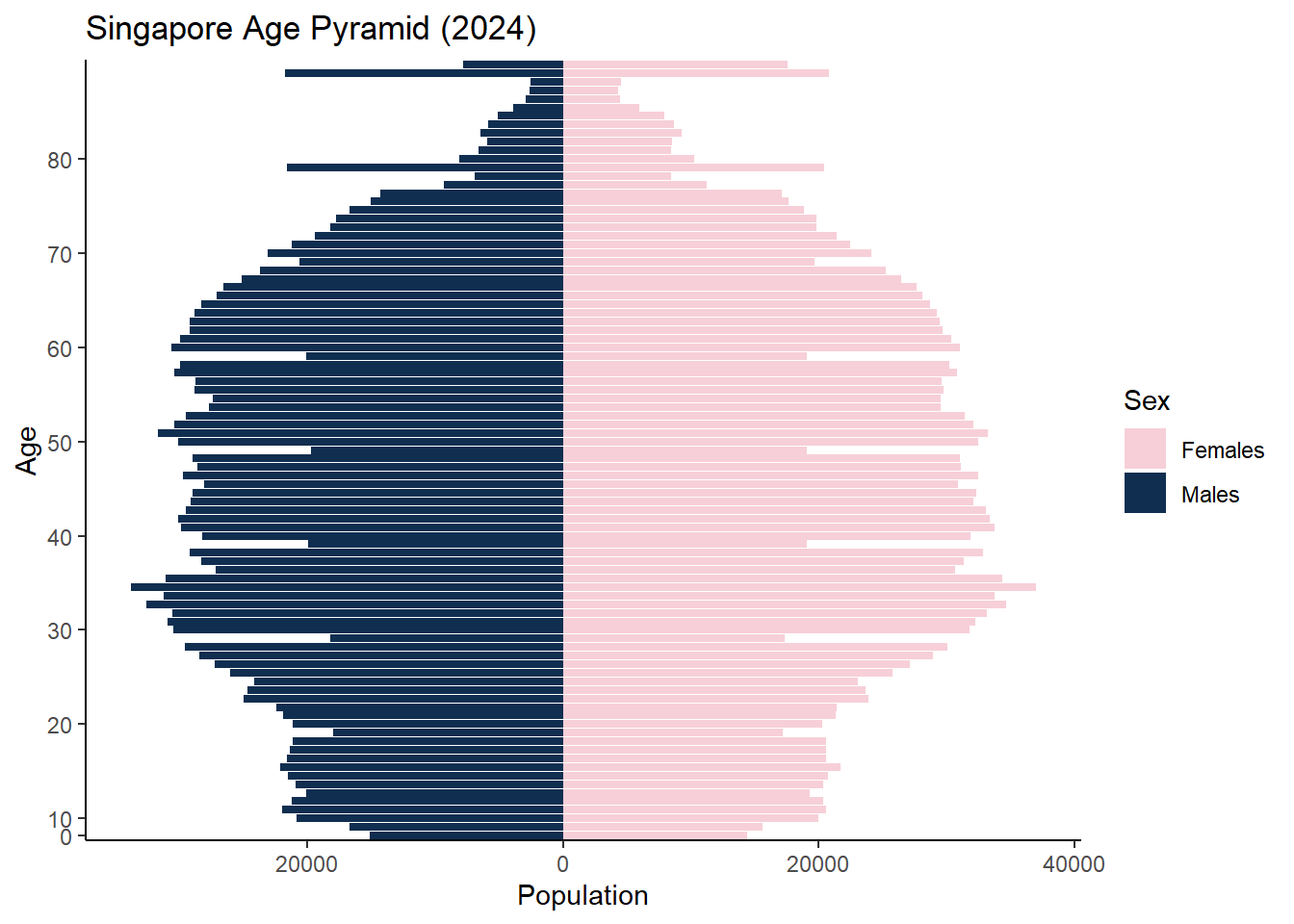

Findings for Figure 1

The age pyramid shows a broad base narrowing progressively with age, typical of a developed country.
Females dominate the older age brackets (70+), reflecting longer life expectancy.
The working-age population (30–50) appears stable.

3.2. Top 20 most popular planning areas with elderly population shown

library(tidyverse)

# Summarise total and elderly population by PA
top_areas <- pop_data %>%
  group_by(PA) %>%
  summarise(
    Total = sum(Pop),
    Elderly = sum(Pop[Age >= 65]),
    .groups = "drop"
  ) %>%
  
  top_n(15, Total)  # or 20 if you prefer

# Reshape into long format for grouped bars
plot_data <- top_areas %>%
  pivot_longer(cols = c(Total, Elderly),
               names_to = "Type",
               values_to = "Population") %>%
  mutate(
    Type = recode(Type,
                  "Total" = "Total Population",
                  "Elderly" = "Elderly (65+)")
  )
# Reorder PA by Total Population (not elderly)
plot_data <- plot_data %>%
  left_join(top_areas %>% select(PA, Total), by = "PA") %>%
  mutate(PA = fct_reorder(PA, Total, .desc = FALSE))  # use forcats::fct_reorder

ggplot(plot_data, aes(x = PA, y = Population, fill = Type)) +
  geom_col(position = "dodge") +
  geom_text(aes(label = scales::comma(Population)),
            position = position_dodge(width = 0.9), hjust = -0.1, size = 3) +
  scale_y_continuous(labels = scales::comma,
                     expand = expansion(mult = c(0, 0.15))) +
  scale_fill_manual(values = c("Total Population" = "#8E7DBE", "Elderly (65+)" = "#EFC000")) +
  coord_flip() +
  labs(
    title = "Total vs Elderly Population in Top Planning Areas (2024)",
    x = "Planning Area",
    y = "Population",
    fill = ""
  ) +
  theme_classic()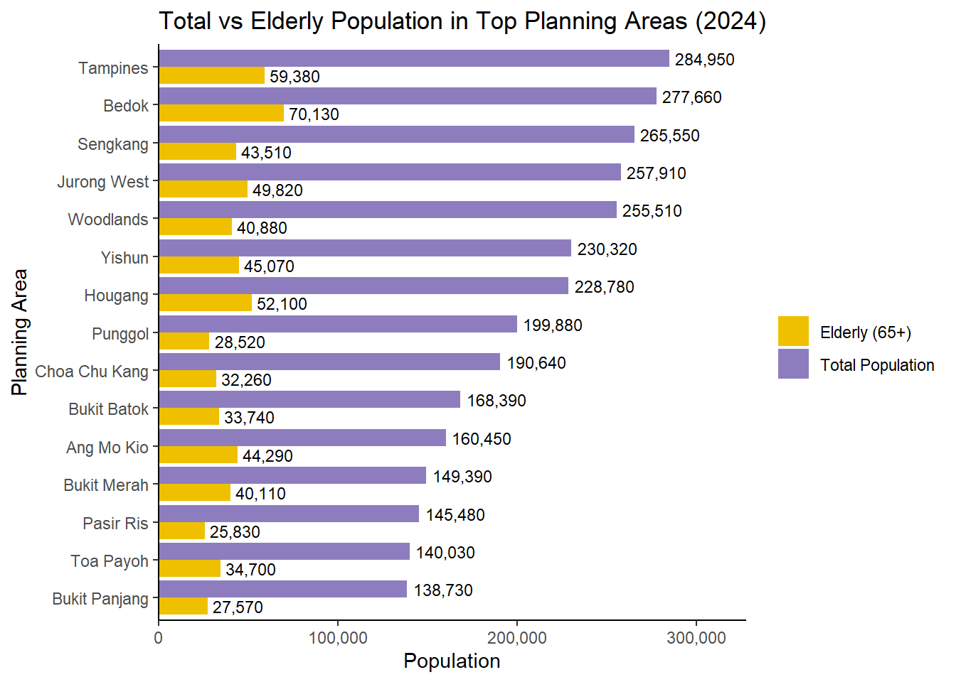

Findings for Figure 2

Tampines, Bedok, and Sengkang have the largest total populations.
Bedok stands out with ~70,000 elderly residents.
Punggol has a younger demographic despite its size.

3.3. Elderly Population Share (%) by Planning Area

elderly_pct_data <- pop_data %>%
  group_by(PA) %>%
  summarise(
    Elderly = sum(Pop[Age >= 65]),
    Total = sum(Pop),
    .groups = "drop"
  ) %>%
  mutate(ElderlyPct = Elderly / Total * 100) %>%
  arrange(desc(ElderlyPct)) %>%
  slice_head(n = 20)  # or more, depending on your needs

ggplot(elderly_pct_data, aes(x = reorder(PA, ElderlyPct), y = ElderlyPct)) +
  geom_col(fill = "#EFC000") +
  coord_flip() +
  labs(
    title = "Top Planning Areas by Elderly Share (%)",
    x = "Planning Area",
    y = "Elderly Population (%)"
  ) +
  theme_classic()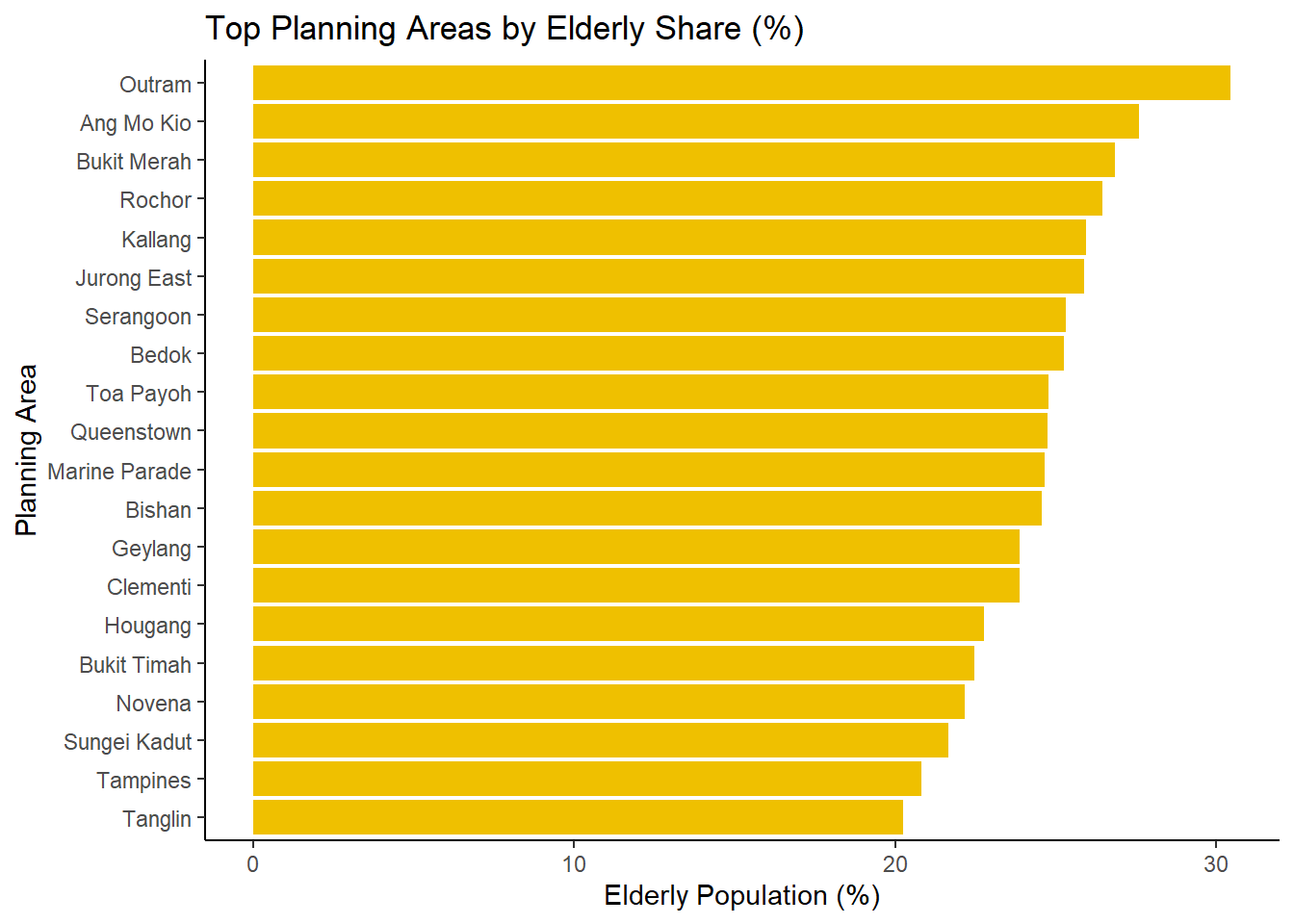

Findings for Figure 3

Outram, Ang Mo Kio, and Bukit Merah have the highest elderly population shares, each with over 25% of their residents aged 65 and above.
Central and mature estates (e.g., Rochor, Toa Payoh, Queenstown) consistently appear in the top rankings for elderly proportion, highlighting the ageing nature of Singapore’s older housing estates.
In contrast, larger but newer areas like Tampines and Punggol have lower elderly shares (below 20%), indicating a younger overall population.

4. Conclusion

The analysis of Singapore’s 2024 demographic structure highlights several key findings:

Balanced Gender Distribution: The national age pyramid shows a fairly balanced distribution between males and females across most age groups, though the female population dominates at older ages (70+), reflecting longer life expectancy among women. ️
High Elderly Counts in Large Towns: Tampines, Bedok, and Sengkang have the largest total populations and also significant absolute numbers of elderly residents (e.g., Bedok: ~70,000 aged 65+). This suggests that elderly care demand is not only in older towns but also in larger ones.
Ageing Hotspots: When measured by the proportion of elderly (65+), smaller central areas like Outram, Ang Mo Kio, and Bukit Merah show the highest elderly shares (over 25% of their populations). These are mature estates that may require priority attention for ageing-in-place policies.

5. Reference

Singapore Residents by Planning Area / Subzone, Single Year of Age and Sex, June 2024

TAKE-HOME EXERCISE 01 - PHASE 2

1. The task

Selecting one submission provided by your classmate, critic three good design principles and three areas for further improvement. With reference to the comment, prepare the makeover version of the data visualization.

My peer’s work

2. Comments on the Work

2.1. Three Good Design Principles

Clear Narrative & Structure The submission provides a clear introduction, context, and explanation for each chart, ensuring the reader understands the purpose of the visualizations. Sections are well-organized with descriptive headings (e.g., “Top 28 Planning Areas by Total Population”).
Effective Chart Titles & Labels Each chart includes concise titles, axis labels, and legends, which make it very easy to interpret the visuals at a glance. The population counts are also nicely formatted (e.g., using commas).
Consistent Styling & Theme The use of a consistent minimal theme (theme_minimal()) and a cohesive color scheme across charts (e.g., blue for males, red/pink for females) helps maintain a professional and unified look.

2.2. Three Areas for Improvements

Color Accessibility While the color scheme is clean, the blue and pink/red tones might be hard to distinguish for colorblind users. Using a colorblind-friendly palette (e.g., via viridis or RColorBrewer) would make the charts more inclusive.
Chart Density & Layout The combined plot (Section 3.1.3) has a large white gap between the two charts (because of the spacer in plot_layout()). This disrupts visual flow. The layout could be improved by: Placing the charts side by side if space allows, Or reducing the spacer height for a tighter design.
Population Pyramid Facet Scaling In the population pyramids (Section 3.2), the facet_wrap uses scales = “free_y”, causing inconsistent y-axis scales across facets. This makes it harder to compare populations between areas. Using a fixed y-scale or at least adding annotations explaining the difference would improve interpretability.

2.3. Makeover Version of the data visualization

Improved Layout for Combined Plot

sg_res <- pop_data

# Original code
top_24_pas <- sg_res %>%
  group_by(PA) %>%
  summarise(Total = sum(Pop), .groups = "drop") %>%
  slice_max(order_by = Total, n = 24) %>%
  pull(PA)

pyramid_data_top24 <- sg_res %>%
  filter(PA %in% top_24_pas) %>%
  group_by(PA, Age, Sex) %>%
  summarise(Pop = sum(Pop), .groups = "drop") %>%
  mutate(
    Age = ifelse(Age == "90_and_Over", 90, as.numeric(Age)),
    Pop = ifelse(Sex == "Males", -Pop, Pop)
  )

Warning: There was 1 warning in `mutate()`.
ℹ In argument: `Age = ifelse(Age == "90_and_Over", 90, as.numeric(Age))`.
Caused by warning in `ifelse()`:
! NAs introduced by coercion

# Get max pop for consistent y-axis
max_pop <- pyramid_data_top24 %>%
  group_by(PA) %>%
  summarise(total = sum(Pop)) %>%
  pull(total) %>%
  max()

# Makeover plot
pyramid_makeover <- ggplot(pyramid_data_top24, aes(x = Age, y = Pop, fill = Sex)) +
  geom_bar(stat = "identity", width = 0.8) +
  coord_flip() +
  scale_y_continuous(labels = abs, limits = c(-max_pop, max_pop)) +  # Fix y-axis scale
  facet_wrap(~PA, scales = "fixed", ncol = 6) +
  labs(
    title = "Population Pyramids of Top 24 Planning Areas (Consistent Y-Axis)",
    x = "Age Group",
    y = "Population"
  ) +
  theme_minimal(base_size = 9) +
  theme(
    axis.title.x = element_text(size = 18),
    axis.title.y = element_text(size = 18),
    plot.title = element_text(size = 24)
  ) +
  scale_fill_viridis_d(option = "D", begin = 0.2, end = 0.8)

print(pyramid_makeover)