pacman::p_load(readxl, gifski, gapminder,
plotly, gganimate, tidyverse)Hands-on Exercise 3B - Programming Animated Statistical Graphics with R
3.1. Getting Started
3.1.1. Loading the packages
3.1.2. Importing the data
col <- c("Country", "Continent")
globalPop <- read_xls("C:/Cindy-2312/ISSS608-VAA/Hands-on_Exercise/Hands-on_Ex03/data/GlobalPopulation.xls",
                      sheet = "Data") %>%
  mutate(across(all_of(col), as.factor)) %>%
  mutate(Year = as.integer(Year))
3.2. Animated data visualisation: gganimate methods
3.2.1. Building a static population bubble plot
ggplot(globalPop, aes(x = Old, y = Young,
                      size = Population,
                      colour = Country)) +
  geom_point(alpha = 0.7,
             show.legend = FALSE) +
  scale_colour_manual(values = country_colors) +
  scale_size(range = c(2, 12)) +
  labs(title = 'Year: {frame_time}',
       x = '% Aged',
y = '% Young') 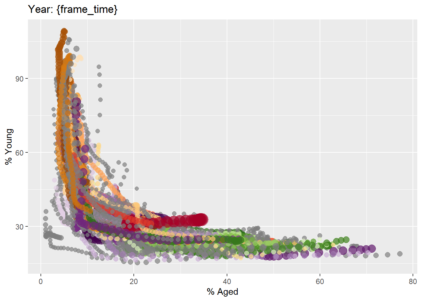
3.2.2. Building the animated bubble plot
ggplot(globalPop, aes(x = Old, y = Young,
                      size = Population,
                      colour = Country)) +
  geom_point(alpha = 0.7,
             show.legend = FALSE) +
  scale_colour_manual(values = country_colors) +
  scale_size(range = c(2, 12)) +
  labs(title = 'Year: {frame_time}',
       x = '% Aged',
       y = '% Young') +
  transition_time(Year) +
ease_aes('linear') 
3.3. Animated data visualisation: plotly
3.3.1. Building an animated bubble plot: ggplotly() method
gg <- ggplot(globalPop,
       aes(x = Old,
           y = Young,
           size = Population,
           colour = Country)) +
  geom_point(aes(size = Population
                ),
             alpha = 0.7,
             show.legend = FALSE) +
  scale_colour_manual(values = country_colors) +
  scale_size(range = c(2, 12)) +
  labs(x = '% Aged',
       y = '% Young')

ggplotly(gg)
3.3.2. Building interactive, animated bubble chart using plotly()
bp <- globalPop %>%
  plot_ly(x = ~Old,
          y = ~Young,
          size = ~Population,
          color = ~Continent,
          sizes = c(2, 100),
          frame = ~Year,
          text = ~Country,
          hoverinfo = "text",
          type = 'scatter',
          mode = 'markers'
          ) %>%
  layout(showlegend = FALSE)
bp